Data Types & Structures
Types of data
R has different types of data, and an object’s type affects how it interacts with functions and other objects.
Types of data
R has different types of data, and an object’s type affects how it interacts with functions and other objects.
So far, we’ve just been working with numeric data, but there are several other types to be aware of...
Types of data
R has different types of data, and an object’s type affects how it interacts with functions and other objects.
So far, we’ve just been working with numeric data, but there are several other types to be aware of...
| Type | Definition | Example |
|---|---|---|
| Integer | whole numbers from -Inf to +Inf | 1L, -2L |
| Double | numbers, fractions & decimals | -7, 0.2, -5/2 |
| Character | quoted strings of letters, numbers, and allowed symbols | "1", "one", "o-n-e", "o.n.e" |
| Logical | logical constants of true or false | TRUE, FALSE |
| Factor | ordered, labelled variable | variable for year in college labelled "Freshman", "Sophomore", etc. |
Types of data
You can use typeof() to find out the type of a value or object
Types of data
You can use typeof() to find out the type of a value or object
typeof(1)## [1] "double"typeof(TRUE)## [1] "logical"typeof(1L)## [1] "integer"typeof("one")## [1] "character"Types of data
There are a few special values worth knowing about too
| Value | Definition |
|---|---|
NA |
Missing value ("not available") |
NaN |
Not a Number (e.g. 0/0) |
Inf |
Positive infinity |
-Inf |
Negative infinity |
NULL |
An object that exists but is completely empty |
Data structures
Vectors
Often, we’re not working with individual values, but with a group of multiple related values -- or a vector of values.
Vectors
Often, we’re not working with individual values, but with a group of multiple related values -- or a vector of values.
We can create a vector of ordered numbers using the form
starting_number : ending_number.
Vectors
Often, we’re not working with individual values, but with a group of multiple related values -- or a vector of values.
We can create a vector of ordered numbers using the form
starting_number : ending_number.
For example, we could make x a vector with the numbers between 1 and 5.
x <- 1:5x## [1] 1 2 3 4 5Vectors
Often, we’re not working with individual values, but with a group of multiple related values -- or a vector of values.
We can create a vector of ordered numbers using the form
starting_number : ending_number.
For example, we could make x a vector with the numbers between 1 and 5.
x <- 1:5x## [1] 1 2 3 4 5Let's look at the Environment pane in RStudio...
Since x is a vector, it tells us what type of vector it is and its length in addition to its contents (which can be abbreviated if the object is larger).
Vectors
We can create a vector of any numbers we want using c(), which is a function. You can think of c() as short for "combine".
Vectors
We can create a vector of any numbers we want using c(), which is a function. You can think of c() as short for "combine".
You use c() by putting numbers separated by a comma within the parentheses.
# combine values into a vector and assign to an object names 'x'x <- c(2, 8.5, 1, 9)# print xx## [1] 2.0 8.5 1.0 9.0Vectors
We can create a vector of any numbers we want using c(), which is a function. You can think of c() as short for "combine".
You use c() by putting numbers separated by a comma within the parentheses.
# combine values into a vector and assign to an object names 'x'x <- c(2, 8.5, 1, 9)# print xx## [1] 2.0 8.5 1.0 9.0We can also create a vector of numbers using seq().
seq() is a function that creates a sequence of numbers.
Vectors
To learn how any R function works, you can access the help documentation by typing ?function_name.
Vectors
To learn how any R function works, you can access the help documentation by typing ?function_name.
Let's take a look at how seq() works...
?seqVectors
What happens if we run seq() with no arguments?
seq()## [1] 1Vectors
What happens if we run seq() with no arguments?
seq()## [1] 1The seq() function has arguments with default values.
The first two arguments are from and to, which specify the starting and end values of the sequence. By default from = 1 and to = 1.
This means that typing seq() is equivalent to typing seq(from = 1, to = 1), which generates a sequence with just one value: 1.
We will talk more about how functions work in the next slide deck.
Vectors
To make a sequence from 1 to 5 with this function, we have to set the arguments accordingly: from = 1 and to = 5
seq(from = 1, to = 5)## [1] 1 2 3 4 5Vectors
To make a sequence from 1 to 5 with this function, we have to set the arguments accordingly: from = 1 and to = 5
seq(from = 1, to = 5)## [1] 1 2 3 4 5We can also set one or more of the other arguments...
Vectors
To make a sequence from 1 to 5 with this function, we have to set the arguments accordingly: from = 1 and to = 5
seq(from = 1, to = 5)## [1] 1 2 3 4 5We can also set one or more of the other arguments...
The by argument allows us to change the increment of the sequence. For example, to get every other number between 1 and 5, we would set by = 2
seq(from = 1, to = 5, by = 2)## [1] 1 3 5Vectors
Vectors are just 1-dimensional sequences of a single type of data.
Vectors
Vectors are just 1-dimensional sequences of a single type of data.
Note that vectors can also include strings or character values.
letters <- c("a", "b", "c", "d")letters## [1] "a" "b" "c" "d"Vectors
Vectors are just 1-dimensional sequences of a single type of data.
Note that vectors can also include strings or character values.
letters <- c("a", "b", "c", "d")letters## [1] "a" "b" "c" "d"The general rule R uses is to set the vector to be the most "permissive" type necessary.
Vectors
Vectors are just 1-dimensional sequences of a single type of data.
Note that vectors can also include strings or character values.
letters <- c("a", "b", "c", "d")letters## [1] "a" "b" "c" "d"The general rule R uses is to set the vector to be the most "permissive" type necessary.
For example, what happens if we combine the vectors x (from earlier) and letters together?
mixed_vec <- c(x, letters)mixed_vec## [1] "2" "8.5" "1" "9" "a" "b" "c" "d"Vectors
mixed_vec## [1] "2" "8.5" "1" "9" "a" "b" "c" "d"Notice the quotes? R turned all of our numbers into strings, since strings are more "permissive" than numbers.
Vectors
mixed_vec## [1] "2" "8.5" "1" "9" "a" "b" "c" "d"Notice the quotes? R turned all of our numbers into strings, since strings are more "permissive" than numbers.
typeof(mixed_vec)## [1] "character"Vectors
mixed_vec## [1] "2" "8.5" "1" "9" "a" "b" "c" "d"Notice the quotes? R turned all of our numbers into strings, since strings are more "permissive" than numbers.
typeof(mixed_vec)## [1] "character"This is called coercion. R coerces a vector into whichever type will accommodate all of the values. We can coerce mixed_vec to be numeric using as.numeric(), but notice what happens to the character values 👀
as.numeric(mixed_vec)## Warning: NAs introduced by coercion## [1] 2.0 8.5 1.0 9.0 NA NA NA NAYour turn 1
01:30
Create an object called
xthat is assigned the number 8.Create an object called
ythat is a sequence of numbers from 2 to 16, by 2.Add
xandy. What happens?
Solution
# Q1.x <- 8# Q2.y <- seq(from = 2, to = 16, by = 2)y## [1] 2 4 6 8 10 12 14 16# Q3x + y## [1] 10 12 14 16 18 20 22 24This is an example of vector recycling.
When applying an operation to two vectors that requires them to be the same length, R automatically recycles, or repeats, the shorter one, until it is long enough to match the longer one.
Your turn 2
03:00
Create an object called
athat is just the letter "a" and an objectxthat is assigned the number 8. Addatox. What happens?Create a vector called
bthat is just the number 8 in quotes. Addbtox(from above). What happens?Find some way to add
btox. (Hint: Don't forget about coercion.)
Indexing vectors
How do we extract elements out of vectors?
Indexing vectors
How do we extract elements out of vectors?
This is called indexing, and it is frequently quite useful
Indexing vectors
How do we extract elements out of vectors?
This is called indexing, and it is frequently quite useful
There are a number of methods for indexing that are good to be familiar with
Indexing vectors
Indexing by position
Vectors can be indexed numerically, starting with 1 (not 0). We can extract specific elements from a vector by putting the index of their position inside brackets [].
Indexing vectors
Indexing by position
Vectors can be indexed numerically, starting with 1 (not 0). We can extract specific elements from a vector by putting the index of their position inside brackets [].
Let's take a new vector z as an example:
z <- 6:10Indexing vectors
Indexing by position
Vectors can be indexed numerically, starting with 1 (not 0). We can extract specific elements from a vector by putting the index of their position inside brackets [].
Let's take a new vector z as an example:
z <- 6:10Let's get just the first element of z:
z[1]## [1] 6Get the first and third element by passing those indexes as a vector using c().
z[c(1, 3)]## [1] 6 8Indexing Vectors
Negative indexing
z## [1] 6 7 8 9 10We could also say which elements not to give us using the minus sign (-).
Indexing Vectors
Indexing by name
Finally, if the elements in the vector have names, we can refer to them by name instead of their numerical index. You can see the names of a vector using names().
names(z)## NULLIndexing Vectors
Indexing by name
Finally, if the elements in the vector have names, we can refer to them by name instead of their numerical index. You can see the names of a vector using names().
names(z)## NULLLooks like the elements in z have no names. We can change that by assigning them names using a vector of character values.
names(z) <- c("first", "second", "third", "fourth", "fifth")z## first second third fourth fifth ## 6 7 8 9 10Indexing Vectors
Indexing by name
z## first second third fourth fifth ## 6 7 8 9 10Now we can use the names of the elements in z for subsetting, using quotes
z["first"]## first ## 6Modifying Vectors
You can use indexing to change elements within a vector.
For example, we could change the first element of z to missing, or NA.
z[1] <- NAz## first second third fourth fifth ## NA 7 8 9 10Your turn 3
03:00
Create a vector called
namedthat includes the numbers 1 to 5. Name the values "a", "b", "c", "d", and "e" (in order).Print the first element using numerical indexing and the last element using name indexing.
Change the third element of
namedto the value 21 and then show your results.
Solution
# Q1. named <- c(a = 1, b = 2, c = 3, d = 4, e = 5)named## a b c d e ## 1 2 3 4 5# this works toonamed <- c(1, 2, 3, 4, 5)names(named) <- c("a", "b", "c", "d", "e")named## a b c d e ## 1 2 3 4 5named[1]## a ## 1named["e"]## e ## 5# Q2.named[3] <- named[3]*7named## a b c d e ## 1 2 21 4 5# this works toonamed[3] <- 21Lists
Vectors are great for storing a single type of data, but what if we have a variety of different kinds of data we want to store together?
Lists
Vectors are great for storing a single type of data, but what if we have a variety of different kinds of data we want to store together?
For example, let's say I have some information about Jane Doe that I want to store together in a single object:
- her name ("Jane Doe") -- a string
- her height in feet (5.5) -- a number
- whether or not she is right-handed (TRUE) -- a logical
A vector won't work -- every element is coerced to a character (notice the quotes).
c("Jane Doe", 5.5, TRUE)## [1] "Jane Doe" "5.5" "TRUE"Lists
Vectors are great for storing a single type of data, but what if we have a variety of different kinds of data we want to store together?
For example, let's say I have some information about Jane Doe that I want to store together in a single object:
- her name ("Jane Doe") -- a string
- her height in feet (5.5) -- a number
- whether or not she is right-handed (TRUE) -- a logical
A vector won't work -- every element is coerced to a character (notice the quotes).
c("Jane Doe", 5.5, TRUE)## [1] "Jane Doe" "5.5" "TRUE"Instead, we can put them in a list. Lists are very flexible -- they can contain different types of data and preserve those types.
Creating Lists
We can create a list with the list() function
Creating Lists
We can create a list with the list() function
jane_doe <- list("Jane Doe", 5.5, TRUE)jane_doe## [[1]]## [1] "Jane Doe"## ## [[2]]## [1] 5.5## ## [[3]]## [1] TRUECreating Lists
And, we can give each element of the list a name to make it easier to keep track of them.
jane_doe <- list(name = "Jane Doe", height = 5.5, right_handed = TRUE)jane_doe## $name## [1] "Jane Doe"## ## $height## [1] 5.5## ## $right_handed## [1] TRUECreating Lists
And, we can give each element of the list a name to make it easier to keep track of them.
jane_doe <- list(name = "Jane Doe", height = 5.5, right_handed = TRUE)jane_doe## $name## [1] "Jane Doe"## ## $height## [1] 5.5## ## $right_handed## [1] TRUENotice that [[1]], [[2]], and [[3]], the element indices, have been replaced by the names name, height and right_handed 👀
Creating Lists
You can also see the names of a list by running names() on it
Creating Lists
You can also see the names of a list by running names() on it
names(jane_doe)## [1] "name" "height" "right_handed"Creating Lists
You can also see the names of a list by running names() on it
names(jane_doe)## [1] "name" "height" "right_handed"Lists are even more flexible than we've seen so far. In addition to being of heterogeneous type, each element of a list can be of different lengths.
Creating Lists
Let's add another element to the list about Jane that contains her favorite types of ice cream (she can't choose just one!)
Notice use of c() to create the element ice_cream 👀
jane_doe <- list(name = "Jane Doe", height = 5.5, right_handed = TRUE, ice_cream = c("mint chip", "pistachio"))jane_doe## $name## [1] "Jane Doe"## ## $height## [1] 5.5## ## $right_handed## [1] TRUE## ## $ice_cream## [1] "mint chip" "pistachio"Indexing Lists
Indexing by position
Like vectors, lists can be indexed by their name or their position (numerically).
Indexing Lists
Indexing by position
Like vectors, lists can be indexed by their name or their position (numerically).
For example, if we wanted the height element, we could get it out using its position as the second element of the list:
jane_doe[2]## $height## [1] 5.5Now let's say we want to know Jane's height in inches. Let's see if we can get that by multiplying the height element by 12.
jane_doe[2] * 12## Error in jane_doe[2] * 12: non-numeric argument to binary operatorR is telling us that we supplied a non-numeric argument, i.e. jane_doe[2].
This happened because single bracket indexing on a list returns a list -- but what we need is the contents of the list (in this case, just the number 5.5).
If we want the actual object stored at the first position instead of a list containing that object, we have to use double-bracket indexing list[[i]]:
jane_doe[[2]]## [1] 5.5Notice it no longer has the $height.
In general, a $label is a hint that you're looking at a list (the container) and not just the object stored at that position (the contents).
Now let's see Jane's height in inches.
jane_doe[[2]] * 12## [1] 66Indexing Lists
Indexing by name
The same applies to name indexing. With lists, you can get a list containing the indexed object with single brackets [].
jane_doe["height"]## $height## [1] 5.5And double brackets [[]] can be used to get the contents -- the object stored with that name.
jane_doe[["height"]]## [1] 5.5You can also use list$name to get the object stored with a particular name too. It is equivalent to double brackets, but you don't need quotes
jane_doe$height## [1] 5.5Modifying Lists
Just like vectors, we can change or add elements to our list using indexing.
Modifying Lists
Just like vectors, we can change or add elements to our list using indexing.
Let's save the inches transformation of the height element as height_in.
jane_doe$height_in <- jane_doe$height * 12jane_doe## $name## [1] "Jane Doe"## ## $height## [1] 5.5## ## $right_handed## [1] TRUE## ## $ice_cream## [1] "mint chip" "pistachio"## ## $height_in## [1] 66Your turn 4
03:00
Create a list like
jane_doethat is made up ofname,height,right_handed, andice_cream, but corresponds to information about you.Index your list to print only your name.
Solution
# Q1. (Answers will vary)jane_doe <- list(name = "Jane Doe", height = 5.5, right_handed = TRUE, ice_cream = c("mint chip", "pistachio"))jane_doe## $name## [1] "Jane Doe"## ## $height## [1] 5.5## ## $right_handed## [1] TRUE## ## $ice_cream## [1] "mint chip" "pistachio"# Q2. jane_doe$name## [1] "Jane Doe"jane_doe[["name"]]## [1] "Jane Doe"Indexing Lists
Indexing objects within lists
As we saw with the object ice_cream stored in the list jane_doe, objects within lists can have different dimensions and length.
Indexing Lists
Indexing objects within lists
As we saw with the object ice_cream stored in the list jane_doe, objects within lists can have different dimensions and length.
What if we wanted just one element of an object in a list, such as just the second element of ice_cream?
Indexing Lists
Indexing objects within lists
As we saw with the object ice_cream stored in the list jane_doe, objects within lists can have different dimensions and length.
What if we wanted just one element of an object in a list, such as just the second element of ice_cream?
We can use indexing on the ice_cream vector stored within the jane_doe list by chaining indexes.
We could do that with numerical indexing...
jane_doe[[4]][2]## [1] "pistachio"...or with name indexing
jane_doe[["ice_cream"]][2]## [1] "pistachio"...or with dollar sign ($) indexing:
jane_doe$ice_cream[2]## [1] "pistachio"Data frames
A data frame is a common way of representing rectangular data -- collections of values that are each associated with a variable (column) and an observation (row). In other words, it has 2 dimensions.
Data frames
A data frame is a common way of representing rectangular data -- collections of values that are each associated with a variable (column) and an observation (row). In other words, it has 2 dimensions.
A data frame is technically a special kind of list -- it can contain different kinds of data in different columns, but each column must be the same length.
We can create a data frame very similarly to how we made a list, but replacing list() with data.frame().
df_1 <- data.frame(c1 = c(1, 3), c2 = c(2, 4), c3 = c("a", "b"))df_1## c1 c2 c3## 1 1 2 a## 2 3 4 bIndexing data frames
df_1## c1 c2 c3## 1 1 2 a## 2 3 4 bIndexing data frames is similar to how we index vectors, except we have two dimensions, which we use like so: [row, column]
Indexing data frames
df_1## c1 c2 c3## 1 1 2 a## 2 3 4 bIndexing data frames is similar to how we index vectors, except we have two dimensions, which we use like so: [row, column]
Let's get the first row and third column of df_1 using numerical indexing
df_1[1, 3]## [1] "a"You can also get an entire row or column by leaving an index blank. Let's get all rows but only column 2:
df_1[, 2]## [1] 2 4We can also index by name
df_1[, "c2"]## [1] 2 4Indexing data frames
df_1## c1 c2 c3## 1 1 2 a## 2 3 4 bAs with lists, we can use the $ operator in the form dataframe$column_name (similar to list$object).
Indexing data frames
df_1## c1 c2 c3## 1 1 2 a## 2 3 4 bAs with lists, we can use the $ operator in the form dataframe$column_name (similar to list$object).
Let's get the first column
df_1$c1## [1] 1 3We can also index a column using vector indexing, since a single column is just a 1-dimensional vector.
df_1$c1[1] # get the first value in column 1## [1] 1Modifying data frames
df_1## c1 c2 c3## 1 1 2 a## 2 3 4 bJust like lists and vectors, you can modify a data frame and add new elements or change existing elements by referencing indexes.
Modifying data frames
df_1## c1 c2 c3## 1 1 2 a## 2 3 4 bJust like lists and vectors, you can modify a data frame and add new elements or change existing elements by referencing indexes.
We could create c4 as the sum of c1 and c2:
df_1$c4 <- df_1$c1 + df_1$c2df_1## c1 c2 c3 c4## 1 1 2 a 3## 2 3 4 b 7
Or we could replace an element using indexing too. Let's replace c1 with c1^2:
df_1$c1 <- df_1$c1^2df_1## c1 c2 c3 c4## 1 1 2 a 3## 2 9 4 b 7Inspecting data frames
df_1## c1 c2 c3 c4## 1 1 2 a 3## 2 9 4 b 7We can use the str() function to get the structure of the data. This tells us the type of each column.
str(df_1)## 'data.frame': 2 obs. of 4 variables:## $ c1: num 1 9## $ c2: num 2 4## $ c3: chr "a" "b"## $ c4: num 3 7Your turn 5
03:00
- Make a data frame, called
df_2, that has 3 columns as shown below. After you create it, check the structure withstr().
## c1 c2 c3## 1 1 2 a## 2 2 4 b## 3 3 6 c- Add a fourth column,
c4, which is the first and second columns multiplied together.
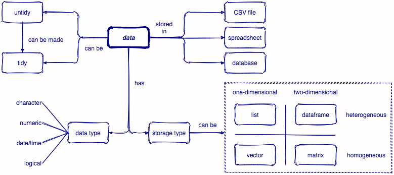
Recap
We just learned about different types of data (numeric, character, logical, factor, etc.) and some different ways they can be structured -- including vectors, lists and data frames.
Recap
We just learned about different types of data (numeric, character, logical, factor, etc.) and some different ways they can be structured -- including vectors, lists and data frames.
Here's a quick table that summarizes data structures.
| Homogeneous data | Heterogeneous data | |
|---|---|---|
| 1-Dimensional | Atomic Vector | List |
| 2-Dimensional | Matrix * |
Data frame |
* We didn't talk about matrices today, but if you take PSY611, you will learn more about them in the context of the General Linear Model
Q & A
05:00
Next up...
Functions & Debugging
Break!
10:00